For Lab 1 of MECE 6397 at the University of Houston, I built a chip thermal simulator from first principles: a 2D transient finite-difference model of a die cross-section with a 700 µm silicon die, a 25 µm grease thermal interface material (TIM) and a 2 mm copper heat spreader cooled from below. The grid is built as a thermal resistance network and marched in time with an explicit forward-Euler scheme. It passed three validation checks against hand physics and was then cross-checked against FiPy, a professional finite-volume solver. On this page you can step through the math and the code, run the same model in your browser and export the result as a GIF.
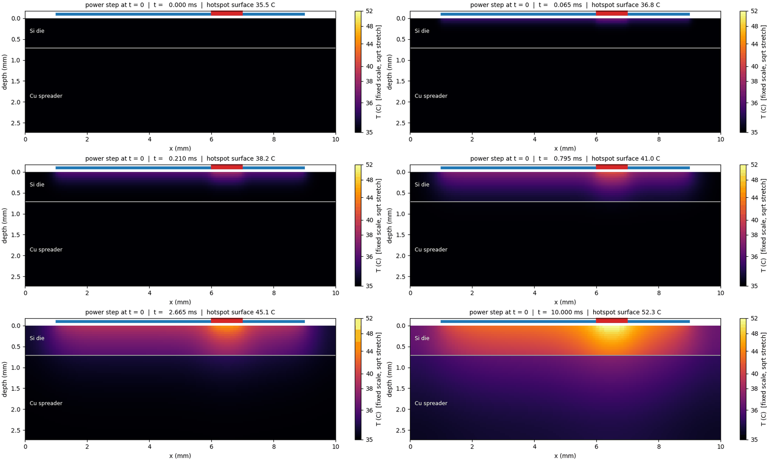
52.3 °C
Hotspot at 10 ms
background 42.9 °C
111.6 °C
Steady hotspot peak
12.1 K above background
101.6 °C
Die-average junction
steady state
0.42 s
Sink time constant
fit (lumped estimate 0.40 s)
The Model
A 10 mm wide slice through a packaged die. The model is 2D, so every quantity is per metre of depth into the page and the hotspot is a 1 mm strip running into the page.
| Layer | Thickness | κ (W/m·K) | ρc (J/m³·K) | In the model |
|---|---|---|---|---|
| Die · Silicon | 700 µm | 148 | 1.63×10⁶ | 14 rows of 50 µm cells |
| TIM · Grease | 25 µm | 5 | 2.0×10⁶ | Interface resistance R″ = 5.0×10⁻⁶ m²K/W |
| Spreader · Copper | 2 mm | 401 | 3.44×10⁶ | 40 rows of 50 µm cells |
Interactive Simulator
The same resistance-network solver, ported from Python to TypeScript, runs on your device. Change the power map, the materials in the stack or the cooling, and the field is re-solved. When you like the result, export it as a GIF.
With the Lab 1 values, this browser version reproduces the Python results: 52.3 °C at the hotspot after 10 ms, 111.6 °C at steady state and a 66.6 K die-average rise. The time step is recomputed from the stability limit for every material choice, and the energy balance is checked on every frame.
Hotspot surface
—
x = 6.50 mm
Background point
—
Hotspot excess
—
peak − background
Energy balance
—
checked every frame
Grid 200 × 54 cells (14 die rows + 40 spreader rows) · Δt = 5.0 µs against a stability limit of 5.36 µs (minimum self-weight 0.067) · 2,000 steps
Export your run as a GIF
Every frame is rendered and encoded on your device, the same way the lab's matplotlib animation was built, with a fixed color scale and a live title.
Math & Thermal Science
These are the core equations behind the simulator, from the governing PDE to the checks that confirmed it was right.
View the equations behind the simulator
Governing physics
Transient conduction in a layered solid, heated on top and cooled from below.
Heat diffusion equation
Energy stored per unit volume equals the net conduction into it. κ changes by a factor of 80 between silicon, grease and copper, so the equation is solved with κ kept inside the divergence.
Boundary conditions
Top: the power map, 100 W/cm² over x = 1–9 mm plus a 200 W/cm² hotspot at 6–7 mm, switched on at t = 0. Bottom: convection with h = 20,000 W/m²K to 35 °C. The sides are adiabatic.
Discretization as a resistance network
Each 50 µm cell is a node: conductances G link neighboring cells and a capacitance C stores energy in each cell.
Conductance and capacitance
Per unit depth, a lateral link through a face of height Δy is κΔy/Δx. With 200 × 54 cells, this gives 10,800 nodes and about 21,300 links.
Explicit (forward-Euler) update
This is the five-point stencil written as a circuit. Q_i = q″Δx is non-zero only in the top row. Every link flow is added to one cell and subtracted from its neighbor, so energy is conserved exactly.
Interfaces and the TIM
Half-cell resistances in series give the harmonic mean of κ across a boundary. The 25 µm grease is only half a cell thick, so it enters as an interface resistance. Its heat capacity (4 % of the die’s) is neglected.
Convective boundary
The bottom node reaches the coolant through half a copper cell plus the film resistance 1/h, a Robin condition written as one more resistor.
Stability of the explicit scheme
Forward Euler is cheap per step, but the time step is capped by the fastest-diffusing material.
Self-weight condition
Copper has the larger diffusivity α = κ/ρc, so it sets the limit. The lab uses Δt = 5.0 µs (mesh number r = 0.233 < 0.25), which takes 2,000 steps for the 0–10 ms window and 800,000 steps to reach steady state at 4 s.
Analytic checks & time scales
Closed-form results the simulation has to reproduce.
Semi-infinite surface heating
Early on, the die behaves like a half-space. At 1 ms, √(αt) = 301 µm, and the simulated surface rise is 2.30 K, matching the 2.30 K given by the formula.
Steady 1-D resistance budget
At P′ = 10 kW per metre of depth, the convective sink takes 74 % of the budget. The full 2D field gives 66.6 K, slightly lower because heat also spreads into the unpowered margins.
Energy audit
Until heat reaches the bottom, all of the input must be stored in the field. The ratio is 1.0000000 at 0.1, 1 and 2 ms.
Two clocks
The die fills with heat in milliseconds, while the spreader and sink take tenths of a second. A fitted late-time exponential gives τ = 0.42 s, two orders of magnitude slower than the die.
Hotspot spreading
A 2D strip can only spread heat sideways, along a logarithmic path. A 45° spreading estimate through the die, TIM and copper (5.9 + 4.2 + 2.4 K) predicts 12.5 K, close to the simulated 12.1 K hotspot excess and about twice the 6 K a real square patch would see. The 2D model is therefore conservative for hotspot design.
Gallery
Click an image to view it full-size.
What the Physics Shows
Heat moves as √(αt)
For the first millisecond the heat stays in a thin surface layer, about 30 µm thick at 10 µs and 300 µm at 1 ms. The spreader does not see the power step until the disturbance reaches the TIM at about 5 ms.
Fast die, slow sink
The 10 ms window captures the die transient but only about a quarter of the eventual rise (17 K of 77 K at the hotspot). Steady state is set by the 0.4 s spreader-and-sink time constant.
The TIM matters most under the hotspot
Hotspot flux has not finished spreading when it reaches the grease, so about a third of the hotspot penalty is lost in just 25 µm of TIM: an 8.8 K jump under the hotspot versus 6.3 K for the average flux.
The sink owns the budget
About 74 % of the steady temperature rise is across the convective sink. A better TIM helps the hotspot, but the junction temperature is mostly set by h.